How to Serve Machine Learning Model using ONNX

6 minute read

In real world machine learning we need more than just predicting single inference, in other words we need low latency for both single or mini batch inference. Unfortunately, most of machine learning frameworks do not provide their model serving frameworks, only some of them do.

In a real world machine learning system, you often need to do more than just run a single inference operation in the REPL or Jupyter notebook. Instead, you usually need to integrate your model into a larger application in some way. Pytorch

Popular libraries such as tensorflow have tensorflow serving which is scalable and most of industries use tensorflow for production. It has low latency, online and batch support, grpc, model management, etc. that is why tensorflow is widely used in the industries.

But what about another popular libraries such as pytorch or xgboost? Data scientist or Machine Learning engineer want to use their favourite library not just single library. In real world machine learning, we should not be fixated on just one machine learning library, we need more diverse. For example:

For GCP we use tensorflow
For research we use pytorch
For AWS we use mxnet
For Azuer we use CNTK
For Apple we use CoreML

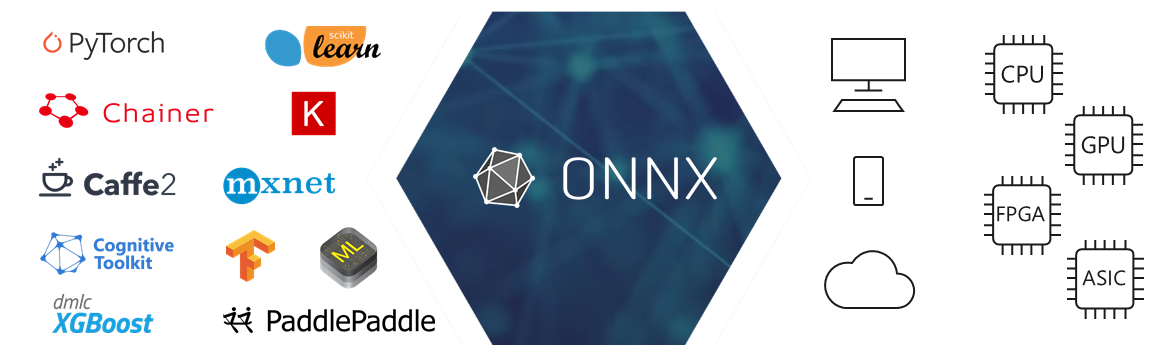
We can exchange the model across library using ONNX

ONNX is an extension of the Open Neural Network Exchange, an open ecosystem that empowers AI developers to choose the right tools as their project evolves. ONNX provides an open source format for AI models, both deep learning and traditional ML. All deep learning libraries can use ONNX to convert to tensorflow so they can use tensorflow serving, but what about traditional machine learning like a tree based algorithm? Although it can be converted into ONNX, but tree based algorithm originating from xgboost or sklearn still cannot be converted to deep learning library (maybe in the future).

no-alignment

Based on that requirements, we need onnx runtime to run onnx inference, even though onnx has compatibility with some runtime like GraphPipe from Oracle which uses flatbuffers or Nvidia with its tensor rt and many more but what I will discuss here is the onnx runtime that comes from onnx itself.

Real world learning machines need more than a single inference. We need low latency in online or mini-batch inferences. In this tutorial I use dataset digits and xgboost to get the model. Full code are available in my repo

Train Model

The code below is a sample code used to train an xgboost model with digits data.

from sklearn.datasets import load_digits
from sklearn.model_selection import train_test_split
import xgboost as xgb

digits = load_digits()
X, y = digits.data, digits.target  # Our train data shape is (x, 64) where x is total samples
X_train, X_test, y_train, y_test = train_test_split(X, y)

booster = xgb.XGBClassifier(max_depth=3,
                            booster='dart',
                            eta=0.3,
                            silent=1,
                            n_estimators=100,
                            num_class=10)

booster.fit(X_train, y_train)

Convert Xgboost to ONNX

After we get the model from xgboost, we can convert the model to onnx with the onnxmltools. For other models you can see it on github.

First, we define the input from the model, this model use float input with shape (1, 64), so we define initial_type as follows.

from onnxmltools.convert.common import data_types

initial_type = [('float_input', data_types.FloatTensorType([1, 64]))]

After that we can immediately change xgboost to onnx using convert_xgboost from onnxmltools and save the model to xgboost.onnx.

from onnxmltools.convert import convert_xgboost

booster_onnx = convert_xgboost(booster, initial_types=initial_type)
onnx.save(booster_onnx, 'xgboost.onnx')

Model Deployment

Model deployment has several approaches, in this post I will discuss direct embedding and microservices.

Direct Embedding

Direct embedding is directly call the model which is as part of the larger program. This case is usually found in the robotic, dedicated devices, or mobile which often calls the model directly as part of the larger program.

Here the code example for direct embedding

import onnxruntime as rt
import numpy as np


test_data = np.random.randint(0, 255, (450, 64))
sess = rt.InferenceSession('xgboost.onnx')

input_name = sess.get_inputs()[0].name
label_name = sess.get_outputs()[0].name
probabilities = sess.get_outputs()[1].name

for x in test_data:
    pred_onx = sess.run([probabilities], {input_name: np.expand_dims(x, axis=0).astype(np.float32)})[0]
    result = {'label': np.argmax(pred_onx), 'probability': max(np.squeeze(pred_onx))}
    print(result)

Microservices

In the other hand if we want to do a management model then we need a separate service that provides an individual model version and usually using package mechanisms such as docker containers and services can be accessed through networks such as JSON over HTTP or rpc technology like grpc. The characteristic of this approach is that you define a service with a single endpoint to call the model then we can do the management model separately.

The first step that must be done is to start the docker container from the onnx runtime server, port 9001 for http and 50051 for grpc while model_path is model_path in the docker

docker run \
    -it \
    -v "$PWD:/models" \
    -p 9001:8001 \
    -p 50051:50051 \
    --name ort mcr.microsoft.com/onnxruntime/server \
    --model_path="/models/xgboost.onnx"

HTTP

For HTTP, then we make a request body first, numpy array will be converted into bytes and predict_pb2 and onnx_ml_pb2 modules are available in my github repo.

import requests

import numpy as np
from google.protobuf.json_format import MessageToJson

import predict_pb2
import onnx_ml_pb2

data = np.random.randint(0, 255, (64))

input_np_array = np.array(data, dtype=np.float32)

input_tensor = onnx_ml_pb2.TensorProto()
input_tensor.dims.extend(input_np_array.shape)
input_tensor.data_type = 1  # float
input_tensor.raw_data = input_np_array.tobytes()

request_message = predict_pb2.PredictRequest()
request_message.inputs['float_input'].data_type = input_tensor.data_type
request_message.inputs['float_input'].dims.extend(input_np_array.shape)
request_message.inputs['float_input'].raw_data = input_tensor.raw_data
request_message = MessageToJson(request_message)

Input from the model is float_input with size (1, 64), data_type = 1 (float32) and you can find another data type from proto file here. Next, we define dimensions (shape) and raw_data in bytes. To get the JSON request body we need to convert from protobuf to JSON with the method MessageToJson.

Then we define the request header.

req_header = {
    'Content-Type': 'application/json',
    'Accept': 'application/x-protobuf'
}

The endpoint URL of the ORT server is http://<your_ip_address>:<port>/v1/models/<your-model-name>/versions/<your-version>:predict

Note: Since we currently only support one model, the model name and version can be any string length > 0. In the future, model_names and versions will be verified.

So, endpoint from our ORT server is http://localhost:9001/v1/models/mymodel/version/1:predict

inference_url = 'http://localhost:9001/v1/models/mymodel/version/1:predict'
response = requests.post(inference_url, headers=req_header, data=request_message)

Response from the ORT server is still in protobuf format, we need to parse it first

If you want to get a response in json, we just need to change req_header to 'Accept': 'application/json'

The following is a way to parse the return protobuf from the ORT server

response_message = predict_pb2.PredictResponse()
response_message.ParseFromString(response.content)

label = np.frombuffer(response.outputs['label'].raw_data, dtype=np.int64)
scores = np.frombuffer(response.outputs['probabilities'].raw_data, dtype=np.float32)

Finally we get label and its probability

GRPC

Same with HTTP until we create request_message

import requests

import numpy as np
from google.protobuf.json_format import MessageToJson

import predict_pb2
import onnx_ml_pb2
import prediction_service_pb2_grpc


data = np.random.randint(0, 255, (64))

input_np_array = np.array(data, dtype=np.float32)

input_tensor = onnx_ml_pb2.TensorProto()
input_tensor.dims.extend(input_np_array.shape)
input_tensor.data_type = 1  # float
input_tensor.raw_data = input_np_array.tobytes()

request_message = predict_pb2.PredictRequest()
request_message.inputs['float_input'].data_type = input_tensor.data_type
request_message.inputs['float_input'].dims.extend(input_np_array.shape)
request_message.inputs['float_input'].raw_data = input_tensor.raw_data

GRPC is available on localhost and port 50051. To call service methods, we first need to create a stub. We instantiate the PredictionServiceStub class of the prediction_service_pb2_grpc module from prediction_service.proto.

with grpc.insecure_channel('localhost:50051') as channel:
    stub = prediction_service_pb2_grpc.PredictionServiceStub(channel)

For RPC methods that return a single response (“response-unary” methods), gRPC Python supports both synchronous (blocking) and asynchronous (non-blocking) control flow semantics A synchronous call to the simple RPC Predict is nearly as straightforward as calling a local method. The RPC call waits for the server to respond, and will either return a response or raise an exception:

response = stub.Predict(request_message)
label = np.frombuffer(response.outputs['label'].raw_data, dtype=np.int64)
scores = np.frombuffer(response.outputs['probabilities'].raw_data, dtype=np.float32)  